Applications in GIS - Module 4 - Coastal Flooding

This week's module for Applications in GIS we were tasked with conducting three different coastal flood analyses. With the use of digital elevation models we delineated coastal flood zones. These analyses utilized both raster and vector data to ultimately achieve our desired result. This lab proved to very challenging for me as I had some issues early on that prohibited me from completing all the steps.

The initial analysis consisted of creating a raster of coastal New Jersey post hurricane Sandy showing erosion and buildup. Below is my map for this analysis where the darkest red shading represents the greatest erosion and the darkest blue represents the areas of the most buildup.

For the final portion of the lab we were tasked with analyzing storm surge in Collier County, Florida. Two DEMs were initially used one by the USGS and another LiDAR derived used to create 1 meter storm surge models. These were to be used to analyze and determine the number of buildings that would be affected by a 1 meter storm surge. Unfortunately, I was unable to complete this objective in its entirety. I was unable to understand the Region Group tool so I skipped it so my data isn't as accurate as it should be. Below is a map showing my two storm surge models.

Overall, this was a challenging model for me because I had some issues understanding some instruction starting in analysis 2. After getting behind I struggled to regroup after becoming frustrated. That said, I was able to get back on track and make some progress with analysis 3 even though I was unable to complete it in its entirety.

Applications in GIS - Module 3 - Visibility Analysis

In this week's module for Applications in GIS, we were introduced to numerous 3D visualization techniques using ArcGIS Pro. Using ArcGIS Pro you can visualize your data in 3D by using a 3D scene. Using 3D scenes can be a powerful tool to enhance the visualization of your data by adding realistic environmental effects making it more attractive to your audience. 

Our assignment for this week was to complete a series of ESRI training courses that introduced us to numerous 3D data visualization techniques. The courses we were assigned included the following courses:

1. Introduction to 3D Visualization

2. Performing Line of Site Analysis

3. Performing Viewshed Analysis in ArcGIS Pro

4. Sharing 3D Content Using Scene Layer Packages 

In the first course, Introduction to 3D Visualization we completed 4 different exercises that taught us about visualizing 3D data in three different views: a map view, a local scene view, or a global scene view. We learned why and when the different views should be utilized, to most effectively display data. We also learned how to determine elevation types, cartographic offset, vertical exaggeration, and extrusion types and methods. The results of a couple of the exercises can be viewed below:

In the above image, we applied realistic enhancements to a downtown San Diego, California local and global scene such as illumination effects, enhanced tree symbology, and detailed buildings.

In the above image, we extruded 2D features by attributes creating a 3D scene. The building parcels shown are not depicted by actual height but rather by property value with yellow representing residential properties, pink commercial properties, and the two gray parcels public housing.

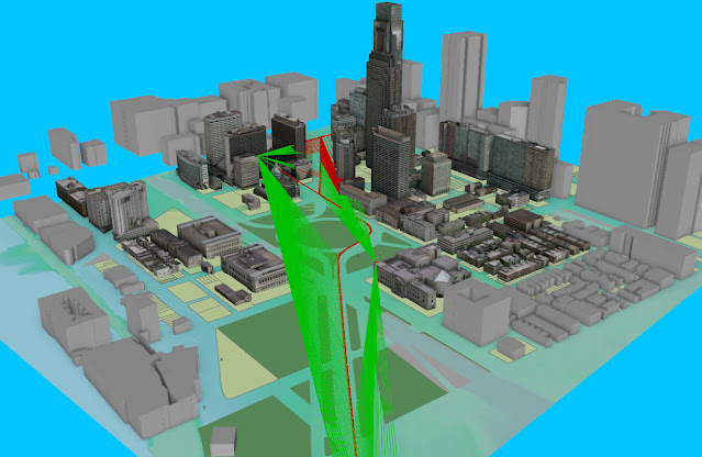
In the second course, Performing Line of Sight Analysis we performed a line of site analysis using a DEM of Philadelphia, Pennsylvania, a parade line, and locations for observers to determine which locations along the route could be observed by security personnel from two observation points. By using ArcGIS 3D analyst tools we were able to determine the optimal line of sight comparing lines greater than 1,100ft and 600ft. Below is a screenshot taken during the process of the analysis.

In the third course, Performing Viewshed Analysis in ArcGIS Pro we created a local scene depicting the hypothetical placement of a new lighting system for a campground in Eastern New York. Using the Viewshed tool, we modeled the range visibility at 3 meters and 10 meters above the surface. Below are the results of the analysis.

The above image shows the results of the 3 meter analysis.

The above image shows the results of the 10 meter analysis.

In the final course, Sharing 3D Content Using Scene Layer Packages we learned how to author a 3D scene using a set of data from the city of Portland, Oregon. Using methods similar to previous courses we converted 2D buildings and trees to 3D features. Our extruded building polygons were converted to multipatch features and the trees were converted to 3D symbology. Finally, we created a scene layer package from our multipatch feature data (the buildings) and published it as a hosted scene layer using ArcGIS Online. Below are two screenshots from the exercises.

The image above depicts the city of Portland global scene with multipatch building features and symbolized trees.

The image above depicts a scene from the published hosted scene layer from ArcGIS Online.


Overall, I really enjoyed these courses and learned a lot of new tools and methods that have provided me with a base knowledge of the 3D visualization capabilities of ArcGIS Pro. 

Applications in GIS - Module 2 - Forestry and Lidar

In the second module for Applications in GIS we were introduced to a more in depth look into LiDAR. LiDAR stands for "Light Detection and Ranging", and while it has been a remote sensing method traditionally used in forestry science, I was first introduced to it while working the field of archaeology. This week's module focused on how LiDAR is applied in forest management and earth science in general.

In this week's lab we worked with LiDAR data from the Shenandoah National Park, Virginia, to examine tree height and tree canopy density.  The LiDAR data we used was obtained from the USGS in the form of an .las file, and then converted to a digital elevation model (DEM). To do this, we used the LAS Dataset to Raster tool in ArcGIS Pro. Next we created a forest height from the DEM and created a map with an accompanying chart showing the tree height. To finish we created a canopy density layer using the LAS to MultiPoint tool, Point to Raster tool, IS NULL tool, Con tool, Plus tool, and finally the Divide tool. 

Below are the maps I created as a result of the data that was generated throughout the process of the lab.

Applications in GIS - Module 1 - Crime Analysis

In the first module for Applications in GIS we were introduced to some mapping techniques employed in crime analysis. These techniques are used to determine hotspots in criminal activity that can be utilized to determine crime rates, identify crime patterns, and compare the reliability of hotspot mapping to predict future crime.

For this module, we were required to create maps using crime data, specifically focusing on homicides in Chicago in 2017 and 2018. Below are three distinct maps illustrating the distribution of homicides in 2017. These maps included: a grid overlay thematic map highlighting areas with the highest 20% of homicides in Chicago, a kernel density map showcasing areas with homicides occurring at three times the mean average, and a local Moran's I map delineating areas aggregated by meaningful boundaries.

Part of the assignment included providing a hypothetical policy recommendation to a police chief on which hotspot map would be the best for predicting future homicides. I would suggest using the Kernel Density map because it would allow for a concentration of resources in areas with the highest density of homicides and has an almost optimal prediction rate. With Kernel Density, one could pinpoint areas with triple the mean homicide rate, whereas with the grid overlay, one could only identify areas in the top 20%. Although Local Moran I's clusters high values within aggregated boundaries, the area might appear broad on the map and could limit police time and resource availability.

Overall, this was a great learning experience that exemplified how GIS principles and technology can be applied to help solve real-world problems. I'm looking forward to learning more GIS applications in the coming modules.

Applications in GIS - About Me Story Map

Hello everyone!

My name is Rick Schmidt and I was born and raised in northwestern Pennsylvania in a small town called Franklin. In 2011, my wife and I relocated to Port Orange, Florida. We have a 6-year-old son (soon to be 7!) that keeps us busy. He is currently interested in learning the principles of engineering and anything outdoors also recently taking an interest in fishing. I joined the UWF graduate certificate program after comparing a handful of programs concluding that UWF was the most robust, offering more than others that I looked into. I earned a bachelor’s degree in anthropology in 2006 from Clarion University of Pennsylvania where I was introduced to GIS through taking an intro class. I was able to apply the skills I learned in that class using ArcMap while employed with the US Forest Service in the Allegheny National Forest where I worked as an archaeologist for three years. 

This is my 5th course in my journey to obtain my GIS graduate certificate here at UWF having just finished the GIS Programming course. Much has changed in the last few months as I ended up accepting a position as an Environmental Scientist at a small environmental firm. I have learned so much through this program and look forward to finishing strong and applying my GIS knowledge in my new position. 

Outside of working and school, I spend time studying the bible, playing basketball and occasionally coaching my son’s sports teams with my wife. In my free time I also enjoy photography as a hobby and volunteer at a local archaeological site in Ormond Beach, Fl. I also serve on the Volusia County Historic Preservation Board.

I look forward to working with everyone this semester!

Here is a link to my StoryMap